Generalized extreme value distribution
| Notation |  |
|---|---|
| Parameters | μ ∈ R — location, σ > 0 — scale, ξ ∈ R — shape. |
| Support | x ∈ [ μ − σ / ξ, +∞) when ξ > 0, x ∈ (−∞, +∞) when ξ = 0, x ∈ (−∞, μ − σ / ξ ] when ξ < 0. |
 where where 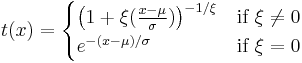 |
|
| CDF |  for x ∈ support for x ∈ support |
| Mean | 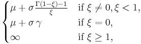 where where  is Euler’s constant. is Euler’s constant. |
| Median | 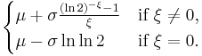 |
| Mode | 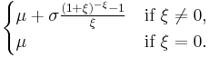 |
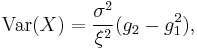
| Variance | 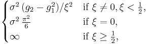 where gk = Γ(1 − kξ). |
| Skewness | 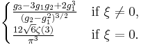 where  is Riemann zeta function is Riemann zeta function |
| Ex. kurtosis | 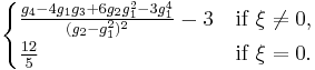 |
| Entropy |  |
| MGF | [1] |
| CF | [1] |
In probability theory and statistics, the generalized extreme value (GEV) distribution is a family of continuous probability distributions developed within extreme value theory to combine the Gumbel, Fréchet and Weibull families also known as type I, II and III extreme value distributions. By the extreme value theorem the GEV distribution is the limit distribution of properly normalized maxima of a sequence of independent and identically distributed random variables. Because of this, the GEV distribution is used as an approximation to model the maxima of long (finite) sequences of random variables.
In some fields of application the generalized extreme value distribution is known as the Fisher–Tippett distribution, named after R. A. Fisher and L. H. C. Tippett who recognised three function forms outlined below. However usage of this name is sometimes restricted to mean the special case of the Gumbel distribution.
Contents |
Specification
The generalized extreme value distribution has cumulative distribution function
![F(x;\mu,\sigma,\xi) = \exp\left\{-\left[1%2B\xi\left(\frac{x-\mu}{\sigma}\right)\right]^{-1/\xi}\right\}](/2012-wikipedia_en_all_nopic_01_2012/I/099a9bb8af60e845e51139f482ea648b.png)
for  , where
  is the location parameter,
  the scale parameter and
  the shape parameter.
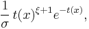
The density function is, consequently
![f(x;\mu,\sigma,\xi) = \frac{1}{\sigma}\left[1%2B\xi\left(\frac{x-\mu}{\sigma}\right)\right]^{(-1/\xi)-1}](/2012-wikipedia_en_all_nopic_01_2012/I/9754f38d985673ab18a0d35f68190916.png)
![\exp\left\{-\left[1%2B\xi\left(\frac{x-\mu}{\sigma}\right)\right]^{-1/\xi}\right\}](/2012-wikipedia_en_all_nopic_01_2012/I/8735fc0f1160b874e38943cc9b1ca476.png)
again, for .
Summary Statistics
Some simple statistics of the distribution are:
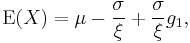
![\operatorname{Mode}(X) = \mu%2B\frac{\sigma}{\xi}[(1%2B\xi)^{-\xi}-1] .](/2012-wikipedia_en_all_nopic_01_2012/I/c97942bda78c84b25415d0d8c7ecadf4.png)
The skewness is for ξ>0
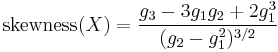
For ξ<0, the sign of the numerator is reversed.
The excess kurtosis is:
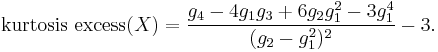
where  , k=1,2,3,4, and
  is the gamma function.
Link to Fréchet, Weibull and Gumbel families
The shape parameter  governs the tail behaviour of the distribution. The sub-families defined by
  ,
,  and
and  correspond, respectively, to the Gumbel, Fréchet and Weibull families, whose cumulative distribution functions are displayed below.
- Gumbel or type I extreme value distribution

- Fréchet or type II extreme value distribution, if ξ=α-1 with

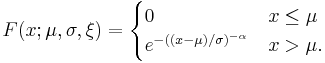
- Reversed Weibull or type III extreme value distribution, if ξ=−α-1, with
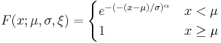
where .
Remark I: The theory here relates to maxima and the distribution being discussed is an extreme value distribution for maxima. A Generalised Extreme Value distribution for minima can be obtained, for example by substituting (-x) for x in the distribution function, and subtracting from one: this yields a separate family of distributions.
Remark II: The ordinary Weibull distribution arises in reliability applications and is obtained from the distribution here by using the variable  , which gives a strictly positive support - in contrast to the use in the extreme value theory here. This arises because the Weibull distribution is used in cases that deal with the minimum rather than the maximum. The distribution here has an addition parameter compared to the usual form of the Weibull distribution and, in addition, is reversed so that the distribution has an upper bound rather than a lower bound. Importantly, in applications of the GEV, the upper bound is unknown and so must be estimated while when applying the Weibull distribution the lower bound is known to be zero.
Remark III: Note the differences in the ranges of interest for the three extreme value distributions: Gumbel is unlimited, Fréchet has a lower limit, while the reversed Weibull has an upper limit.
One can link the type I to types II and III the following way: if the cumulative distribution function of some random variable  is of type II:
  , then the cumulative distribution function of
  is of type I, namely
  . Similarly, if the cumulative distribution function of is of type III: , the cumulative distribution function of is of type I:
  .
.
Properties
The cumulative distribution function of generalized extreme value distribution solves the stability postulate equation. The generalized extreme value distribution is a special case of a max-stable distribution, and is a transformation of a min-stable distribution.
Related distributions
- If
 then
then 
- If
 (Gumbel distribution) then
 - If
 (Weibull distribution) then
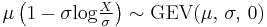
- If then
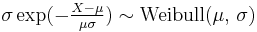 (Weibull distribution)
 - If
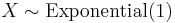 (Exponential distribution) then
See also
Notes
- ^ a b Muraleedharan. G, C. Guedes Soares and Cláudia Lucas (2011). "Characteristic and Moment Generating Functions of Generalised Extreme Value Distribution (GEV)". In Linda. L. Wright (Ed.), Sea Level Rise, Coastal Engineering, Shorelines and Tides, Chapter-14, pp. 269-276. Nova Science Publishers. ISBN 978-1-61728-655-1
References
- Embrechts, P., C. Klüppelberg, and T. Mikosch (1997) Modelling extremal events for insurance and finance. Berlin: Spring Verlag
- Leadbetter, M.R., Lindgren, G. and Rootzén, H. (1983). Extremes and related properties of random sequences and processes. Springer-Verlag. ISBN 0-387-90731-9.
- Resnick, S.I. (1987). Extreme values, regular variation and point processes. Springer-Verlag. ISBN 0-387-96481-9.
- Coles, Stuart (2001). An Introduction to Statistical Modeling of Extreme Values,. Springer-Verlag. ISBN 1-85233-459-2. http://books.google.com/books?id=2nugUEaKqFEC&lpg=PP1&pg=PP1#v=onepage&q=&f=false.